How streaming tables work

/shared/preview.md

A streaming table is a regular Delta table with extra support for streaming or incremental data processing.

Streaming tables are a good choice for data ingestion for the following reasons:

• Each input row is handled only once, which models the vast majority of ingestion workloads (that is, by appending or upserting rows into a table).

• They can handle large volumes of append-only data.

Streaming tables are also a good choice for low-latency streaming transformations for the following reasons:

• Reason over rows and windows of time

• Handle high volumes of data

• Low latency

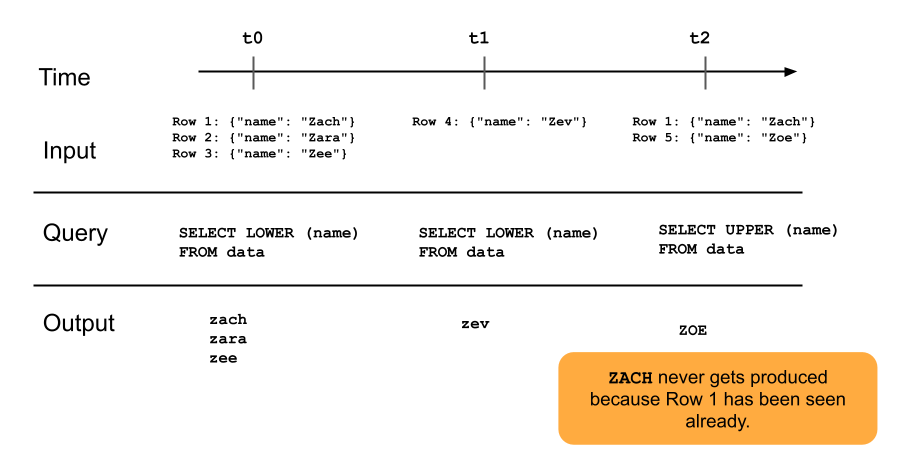
The following diagram illustrates how streaming tables work.

Streaming tables are defined and updated by a single Delta Live Tables pipeline. When you create a Delta Live Tables pipeline, you can explicitly define streaming tables in the source code of the pipeline. These tables are then defined by this pipeline and can’t be changed or updated by any other pipeline. When you create a streaming table in Databricks SQL, Databricks creates a Delta Live Tables pipeline which is used to update this table.

Streaming tables for ingestion

Streaming tables are designed for append-only data sources and process inputs only once.

Full refresh makes streaming tables reprocess data that has already been processed. The full refresh action makes a streaming table reprocess all inputs, including those that have already been processed before.

The following example shows how to use a streaming table to ingest new files from cloud storage. When you use one or more spark.readStream invocations in a dataset definition, it causes Delta Live Tables to treat the dataset as a streaming table instead of a materialized view.

import dlt

@dlt.table
def raw_customers():
  return (
    spark.readStream.format("cloudFiles")
     .option("cloudFiles.format", "json")
     .option("cloudFiles.inferColumnTypes", "true")
     .load("/Volumes/path/to/files")
  )

The following diagram illustrates how append-only streaming tables work.

Streaming tables and low-latency streaming

Streaming tables are designed for low-latency streaming over bounded state. Streaming tables use RocksDB for checkpoint management, which makes them well-suited for low-latency streaming. However, they expect streams that are naturally bounded or bounded with a watermark.

A naturally bounded stream is produced by a streaming data source that has a well-defined start and end. An example of a naturally bounded stream is reading data from a directory of files where no new files are being added after an initial batch of files is placed. The stream is considered bounded because the number of files is finite, and then, the stream ends after all of the files have been processed.

You can also use a watermark to bound a stream. A watermark in Spark Structured Streaming is a mechanism that helps handle late data by specifying how long the system should wait for delayed events before considering the window of time as complete. An unbounded stream that does not have a watermark can cause a Delta Live Tables pipeline to fail due to memory pressure.

Stream-snapshot joins

Stream-snapshot joins are joins between a stream and a dimension that is snapshotted when streams start. These joins do not recompute if the dimension changes after the stream has started, because the dimension table is treated as a snapshot in time, and changes to the dimension table after the stream starts are not reflected unless you reload or refresh the dimension table. This is reasonable behavior if you can accept small discrepancies in a join. For example, an approximate join is acceptable when the number of transactions is many orders of magnitude larger than the number of customers.

In the following code example, we join a dimension table, customers, with two rows with an ever-increasing dataset, transactions. We materialize a join between these two datasets in a table called sales_report. Note that if an outside process updates the customers table by adding a new row (customer_id=3, name=Zoya), this new row will NOT be present in the join because the static dimension table was snapshotted when streams were started.

import dlt

@dlt.view
# assume this table contains an append-only stream of rows about transactions
# (customer_id=1, value=100)
# (customer_id=2, value=150)
# (customer_id=3, value=299)
# ... <and so on> ...
def v_transactions():
  return spark.readStream.table("transactions")

# assume this table contains only these two rows about customers
# (customer_id=1, name=Bilal)
# (customer_id=2, name=Olga)
@dlt.view
def v_customers():
  return spark.read.table("customers")

@dlt.table
def sales_report():
  facts = spark.readStream.table("v_transactions")
  dims = spark.read.table("v_customers")

  return (
    facts.join(dims, on="customer_id", how="inner"
  )

Streaming table limitations

Streaming tables have the following limitations:

• Limited evolution: You can change the query without recomputing the entire dataset. Since a streaming table sees a row only once, you can have different queries operating on different rows. This means you must be aware of all previous versions of the query that are running on your dataset. A full refresh is required to make the streaming table see data that has been seen again.

• State management: Streaming tables are low-latency so you need to ensure that the streams they operate over are naturally bounded or bounded with watermark.

• Joins don’t recompute: Unlike materialized views whose results are always correct because they automatically recompute, joins in streaming tables do not recompute when dimensions change. This characteristic can be good for “fast-but-wrong” scenarios.